Spectral Access

This notebook is one of a set produced by NAVO to demonstrate data access with python tools.

In this notebook, we show how to search for and retrieve spectra from VO services using the Registry and the Simple Spectral Access (SSA) protocol.

import numpy as np

import matplotlib
import matplotlib.pyplot as plt
%matplotlib inline

import requests, io

from astropy.table import Table
import astropy.io.fits as fits
from astropy.coordinates import SkyCoord
# For downloading files
from astropy.utils.data import download_file

import pyvo as vo

# There are a number of relatively unimportant warnings that show up, so for now, suppress them:
import warnings
warnings.filterwarnings("ignore", module="astropy.io.votable.*")
warnings.filterwarnings("ignore", module="pyvo.utils.xml.*")

Finding available Spectral Access Services

First, we find out what spectral access services (‘ssa’) are available in the Registry offering x-ray data.

services = vo.regsearch(servicetype='ssa',waveband='x-ray')
services.to_table()['ivoid','short_name']

Table length=6

ivoid	short_name
object	object
ivo://nasa.heasarc/chanmaster	Chandra
ivo://nasa.heasarc/hitomaster	HITOMASTER
ivo://nasa.heasarc/intbsc	INTEGRAL/BSC
ivo://nasa.heasarc/xtemaster	RXTE
ivo://ned.ipac/sed_data_near_position	NED_SED
ivo://wfau.roe.ac.uk/heavens_at_isdc/light-curves	HEAVENS @ ISDC

We can look at only the Chandra entry:

chandra_service = [s for s in services if 'Chandra' in s.short_name][0]
chandra_service.access_url

'https://heasarc.gsfc.nasa.gov/xamin/vo/ssa?table=chanmaster&'

Chandra Spectrum of Delta Ori

Getting the list of spectra.

delori = SkyCoord.from_name("Delta Ori")

spec_tables = chandra_service.search(pos=delori,diameter=0.1)
spec_tables.to_table().show_in_notebook()

Table length=6

idx	obsid	status	name	ra	dec	time	detector	grating	exposure	type	pi	public_date	datalink	SSA_start_time	SSA_tmid	SSA_stop_time	SSA_duration	SSA_coord_obs	SSA_ra	SSA_dec	SSA_fov	SSA_title	SSA_reference	SSA_datalength	SSA_datamodel	SSA_instrument	SSA_publisher	SSA_format	SSA_wavelength_min	SSA_wavelength_max	SSA_bandwidth	SSA_bandpass	cloud_access
				deg	deg	d			s			d		d	d	d	s	deg	deg	deg	deg								m	m	m	m
0	639	archived	DELTA ORI	83.00125	-0.29917	51556.1364	ACIS-S	HETG	49680	GO	Cassinelli	52037	11172:chandra.obs.misc	51556.136400463	--	--	49680.0	--	83.00125	-0.29917	0.81	acisf00639N004_pha2.fits	https://heasarc.gsfc.nasa.gov/FTP/chandra/data/byobsid/9/639/primary/acisf00639N004_pha2.fits.gz	12	Spectrum-1.0	ACIS-S	HEASARC	application/fits	1.2398e-10	6.1992e-09	6.07522e-09	3.16159e-09	{"aws":{"bucket_name":"nasa-heasarc","region":"us-east-1","policy":"open","key":"chandra/data/byobsid/9/639/primary/acisf00639N004_pha2.fits.gz"}}
1	14570	archived	Delta Ori	83.00167	-0.29908	56285.5508	ACIS-S	HETG	124100	GO	Corcoran	56652	11173:chandra.obs.misc	56285.5507986111	--	--	124100.0	--	83.00167	-0.29908	0.81	acisf14570N003_pha2.fits	https://heasarc.gsfc.nasa.gov/FTP/chandra/data/byobsid/0/14570/primary/acisf14570N003_pha2.fits.gz	12	Spectrum-1.0	ACIS-S	HEASARC	application/fits	1.2398e-10	6.1992e-09	6.07522e-09	3.16159e-09	{"aws":{"bucket_name":"nasa-heasarc","region":"us-east-1","policy":"open","key":"chandra/data/byobsid/0/14570/primary/acisf14570N003_pha2.fits.gz"}}
2	14567	archived	Delta Ori	83.00167	-0.29908	56280.7037	ACIS-S	HETG	116500	GO	Corcoran	56647	11174:chandra.obs.misc	56280.7036921296	--	--	116500.0	--	83.00167	-0.29908	0.81	acisf14567N003_pha2.fits	https://heasarc.gsfc.nasa.gov/FTP/chandra/data/byobsid/7/14567/primary/acisf14567N003_pha2.fits.gz	12	Spectrum-1.0	ACIS-S	HEASARC	application/fits	1.2398e-10	6.1992e-09	6.07522e-09	3.16159e-09	{"aws":{"bucket_name":"nasa-heasarc","region":"us-east-1","policy":"open","key":"chandra/data/byobsid/7/14567/primary/acisf14567N003_pha2.fits.gz"}}
3	14568	archived	Delta Ori	83.00167	-0.29908	56288.1612	ACIS-S	HETG	123600	GO	Corcoran	56655	11175:chandra.obs.misc	56288.1612268519	--	--	123600.0	--	83.00167	-0.29908	0.81	acisf14568N003_pha2.fits	https://heasarc.gsfc.nasa.gov/FTP/chandra/data/byobsid/8/14568/primary/acisf14568N003_pha2.fits.gz	12	Spectrum-1.0	ACIS-S	HEASARC	application/fits	1.2398e-10	6.1992e-09	6.07522e-09	3.16159e-09	{"aws":{"bucket_name":"nasa-heasarc","region":"us-east-1","policy":"open","key":"chandra/data/byobsid/8/14568/primary/acisf14568N003_pha2.fits.gz"}}
4	7416	archived	delta Ori (HD 36486)	83.00167	-0.29908	54413.427	HRC-S	LETG	97080	GO	Raassen	54783	11176:chandra.obs.misc	54413.4270486111	--	--	97080.0	--	83.00167	-0.29908	0.81	hrcf07416N004_pha2.fits	https://heasarc.gsfc.nasa.gov/FTP/chandra/data/byobsid/6/7416/primary/hrcf07416N004_pha2.fits.gz	2	Spectrum-1.0	HRC-S	HEASARC	application/fits	1.2398e-10	6.1992e-09	6.07522e-09	3.16159e-09	{"aws":{"bucket_name":"nasa-heasarc","region":"us-east-1","policy":"open","key":"chandra/data/byobsid/6/7416/primary/hrcf07416N004_pha2.fits.gz"}}
5	14569	archived	Delta Ori	83.00167	-0.29908	56283.254	ACIS-S	HETG	120850	GO	Corcoran	56650	11177:chandra.obs.misc	56283.2539814815	--	--	120850.0	--	83.00167	-0.29908	0.81	acisf14569N003_pha2.fits	https://heasarc.gsfc.nasa.gov/FTP/chandra/data/byobsid/9/14569/primary/acisf14569N003_pha2.fits.gz	12	Spectrum-1.0	ACIS-S	HEASARC	application/fits	1.2398e-10	6.1992e-09	6.07522e-09	3.16159e-09	{"aws":{"bucket_name":"nasa-heasarc","region":"us-east-1","policy":"open","key":"chandra/data/byobsid/9/14569/primary/acisf14569N003_pha2.fits.gz"}}

Accessing one of the spectra.

## If you only run this once, you can do it in memory in one line:
##  This fetches the FITS as an astropy.io.fits object in memory
# hdu_list = spec_tables[0].getdataobj()
## But if you might run this notebook repeatedly with limited bandwidth,
##  download it once and cache it.
file_name = download_file(spec_tables[0].getdataurl(),cache=True)
hdu_list = fits.open(file_name)

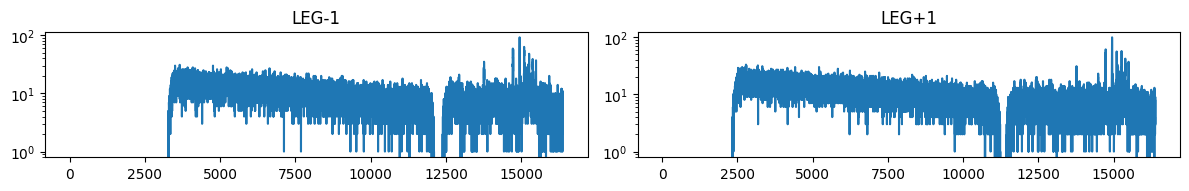
Simple example of plotting a spectrum

spec_table = Table(hdu_list[1].data)
spec_table

Table length=12

SPEC_NUM	TG_M	TG_PART	TG_SRCID	X	Y	CHANNEL	COUNTS	STAT_ERR	BACKGROUND_UP	BACKGROUND_DOWN	BIN_LO	BIN_HI
int16	int16	int16	int16	float32	float32	int16[8192]	int16[8192]	float32[8192]	int16[8192]	int16[8192]	float64[8192]	float64[8192]
1	-3	1	1	4102.815	4131.828	1 .. 8192	0 .. 0	1.8660254 .. 1.8660254	0 .. 0	0 .. 0	7.159166666667378 .. 0.3333333333333333	7.160000000000712 .. 0.33416666666666667
2	-2	1	1	4102.815	4131.828	1 .. 8192	0 .. 0	1.8660254 .. 1.8660254	0 .. 0	0 .. 0	10.738750000000886 .. 0.5	10.740000000000887 .. 0.50125
3	-1	1	1	4102.815	4131.828	1 .. 8192	0 .. 0	1.8660254 .. 1.8660254	0 .. 0	0 .. 0	21.477500000001772 .. 1.0	21.480000000001773 .. 1.0025
4	1	1	1	4102.815	4131.828	1 .. 8192	0 .. 0	1.8660254 .. 1.8660254	0 .. 0	0 .. 0	21.477500000001772 .. 1.0	21.480000000001773 .. 1.0025
5	2	1	1	4102.815	4131.828	1 .. 8192	0 .. 0	1.8660254 .. 1.8660254	0 .. 0	0 .. 0	10.738750000000886 .. 0.5	10.740000000000887 .. 0.50125
6	3	1	1	4102.815	4131.828	1 .. 8192	0 .. 0	1.8660254 .. 1.8660254	0 .. 0	0 .. 0	7.159166666667378 .. 0.3333333333333333	7.160000000000712 .. 0.33416666666666667
7	-3	2	1	4102.815	4131.828	1 .. 8192	0 .. 0	1.8660254 .. 1.8660254	0 .. 0	0 .. 0	13.985000000001373 .. 0.3333333333333333	13.98666666666804 .. 0.33499999999999996
8	-2	2	1	4102.815	4131.828	1 .. 8192	0 .. 0	1.8660254 .. 1.8660254	0 .. 0	0 .. 0	20.977500000001505 .. 0.5	20.980000000001507 .. 0.5025
9	-1	2	1	4102.815	4131.828	1 .. 8192	0 .. 0	1.8660254 .. 1.8660254	0 .. 0	0 .. 0	41.95500000000301 .. 1.0	41.960000000003014 .. 1.005
10	1	2	1	4102.815	4131.828	1 .. 8192	0 .. 0	1.8660254 .. 1.8660254	0 .. 0	0 .. 0	41.95500000000301 .. 1.0	41.960000000003014 .. 1.005
11	2	2	1	4102.815	4131.828	1 .. 8192	0 .. 0	1.8660254 .. 1.8660254	0 .. 0	0 .. 0	20.977500000001505 .. 0.5	20.980000000001507 .. 0.5025
12	3	2	1	4102.815	4131.828	1 .. 8192	0 .. 0	1.8660254 .. 1.8660254	0 .. 0	0 .. 0	13.985000000001373 .. 0.3333333333333333	13.98666666666804 .. 0.33499999999999996

matplotlib.rcParams['figure.figsize'] = (12, 10)

for i in range(len(spec_table)):

    ax = plt.subplot(6,2,i+1)
    pha = plt.plot( spec_table['CHANNEL'][i],spec_table['COUNTS'][i])
    ax.set_yscale('log')

    if spec_table['TG_PART'][i] == 1:
        instr='HEG'
    if spec_table['TG_PART'][i] == 2:
        instr='MEG'
    if spec_table['TG_PART'][i] == 3:
        instr='LEG'

    ax.set_title("{grating}{order:+d}".format(grating=instr, order=spec_table['TG_M'][i]))

    plt.tight_layout()

This can then be analyzed in your favorite spectral analysis tool, e.g., pyXspec. (For the winter 2018 AAS workshop, we demonstrated this in a notebook that you can consult for how to use pyXspec, but the pyXspec documentation will have more information.)